|
|
Contained fluids heated from below spontaneously organize into convection cells when sufficiently far from conductive equilibrium. Fluids can also be organized by surface tension, and other forces and structures at the top, and by imposed horizontal temperature gradients and motions. At mantle conditions rocks are generally treated as fluids. Plate tectonics was once regarded as passive motion of plates on top of mantle convection cells but it now appears that continents and plate tectonics organize the flow in the mantle and that the mantle is the passive element. The flow is driven by instability of the cold surface layer and near-surface lateral temperature gradients such as imposed by slabs and continents. Plate tectonics may be a self-driven, far-from-equilibrium system that organizes itself by dissipation (entropy production) in and between the plates. The mantle may simply be a provider of energy and material. The effect of pressure suppresses the role of the lower thermal boundary layer (TBL) at the core-mantle-boundary (CMB) interface. The state of stress in the lithosphere defines the plates, plate boundaries and locations of midplate volcanism. Fluctuations in stress, due to changing boundary conditions, are responsible for global plate reorganizations and evolution of volcanic chains. In Rayleigh-Benard convection, by contrast, temperature fluctuations are the important parameter. In plume theory, plates break where heated or uplifted by plumes. Ironically, the fluid flows in the experiments by Benard, which motivated the theory by Rayleigh, were driven by surface tension, i.e. stresses at the surface. |
|
|
Mantle convection is quite different from the usual pot-on-a-stove metaphor. A large bowl of several superposed fluids and ice cubes in a microwave oven, programmed to decrease the power with time, would be a better, but still incomplete, analogy. The missing element in laboratory and kitchen experiments, and most computer simulations, is pressure. The mantle is heated from within, cooled from above and cools off with time (secular cooling). All of these effects drive convective motions. The distribution of radioactive elements within the Earth is not uniform. Heating from below is minor, at least for the mantle as a whole. Viscosity varies with depth and temperature. Solid-solid phase changes (some exothermic and some endothermic), occur at various depths. Rheology changes with stress. There are text books, monographs and hundreds of papers on the subject of thermal convection but few are applicable to the mantle. Mantle convection is far from being a closed subject. Computer simulations have not yet included a self-consistent thermodynamic treatment of the effect of temperature, pressure and volume on the physical and thermal properties, and understanding of the “exterior” problem (the surface boundary condition) is in its infancy. Plate tectonics itself is implicated in the surface boundary condition. Melting is an important aspect of real mantle convection. Sphericity, pressure and the distribution of radioactivity break the symmetry of the problem and the top and bottom boundary conditions play quite different roles than in the simple calculations and cartoons of mantle dynamics and geochemical reservoirs. Conventional (Rayleigh-Benard) convection theory may have little to do with plate tectonics. The research opportunities are enormous. |
The history of ideas
Convection can be driven by bottom heating, top or side cooling, and by motions of the boundaries. Although the role of the surface boundary layer and “slab-pull” are now well understood and the latter is generally accepted as the prime mover in plate tectonics, there is a widespread perception that active hot upwellings from deep in the interior of the planet, independent of plate tectonics, are responsible for “extraordinary” events such as plate reorganization, continental break-up, extensive magmatism and events far away from current plate boundaries. Plate tectonics is considered by some to be an incomplete theory of mantle dynamics. Active upwellings from deep in the mantle are viewed as controlling some aspects of surface tectonics and volcanism, including reorganization, implying that the mantle is not passive. These have been modeled by the injection of hot fluids into the base of a tank of motionless fluid. This is called the plume mode of mantle convection.
Numerical experiments show that mantle convection is controlled from the top by continents, cooling lithosphere, slabs and plate motions and that plates not only drive and break themselves but can control and reverse convection in the mantle (1-6). Supercontinents and other large plates generate spatial and temporal temperature variations. The migration of continents, ridges and trenches cause a constantly changing surface boundary condition, and the underlying mantle responds passively (7-10). Plates break up and move, and trenches roll back because of forces on the plates and interactions of the lithosphere with the mantle. Density variations in the mantle are, by and large, generated by plate tectonics itself, for example through slab cooling, refertization of the mantle, continental insulation, and these also affect the forces on the plates. Surface plates are constantly evolving and reorganizing although major reorganizations are infrequent. They are mainly under lateral compression although local regions having horizontal least-compressive axes may be the locus of dikes and volcanic chains.
The mantle is generally considered to convect as a single layer (whole mantle convection) or, at most two (the standard geochemical model). However, the mantle is more likely to convect in multiple layers as a result of gravitational sorting during accretion and the density difference between the mantle products of differentiation. |
 Cross section through the whole-mantle tomography model of Ritsema et al. (1999) showing the strong heterogeneity that characterises the upper mantle and the core-mantle boundary region, contrasting with the weak heterogeneity in the mid-mantle. The mantle may be divided into three or more chemically distinct layers.
 |
Boundary Conditions
The core has low viscosity and high thermal conductivity so the base of the mantle is in contact with a stress-free isothermal bath. The top boundary condition is plate tectonics. It is not an isothermal, stress-free, homogeneous, uniform boundary condition. If the plates are held together by lateral stress (7-10) then the surface must be free to self-organize, a condition not yet allowed in any simulation. Reorganization means the ability to form new plate boundaries and generate new plates that are consistent with the ever-changing stress state of the lithosphere. In the absence of plates or a high viscosity lid the mantle would experience Rayleigh-Benard convection. Above a critical Rayleigh number fluids spontaneously convect and self-organize. Buoyancy of the fluid, which is dependent on the coefficient of thermal expansion (expansivity) and temperature fluctuations, drives the flow and the viscosity forces of the fluid dissipate the energy. Temperature-dependent viscosity, a semi-rigid lithosphere (held together by lateral compressive stresses) and buoyant continents (and thick crust regions) completely change this. Gravitational forces on cooling plates cause them to move. Dissipation takes place in and between the plates, causing them to self-organize and to organize the underlying weaker mantle.
Plate tectonics, to a large extent, is driven by the unstable surface TBL and therefore resembles convection in fluids which are cooled from above (see http://anquetil.colorado.edu/VE/convection.shtml). Pressure decreases the expansivity and Rayleigh number so it is difficult to generate buoyancy or vigorous small-scale convection at the base of the mantle. In addition, heat flow across the CMB is about an order of magnitude less than at the surface so it takes a long time to build up buoyancy. In contrast to the upper TBL, which involves frequent ejections of narrow dense slabs into the interior, the lower TBL is sluggish and does not play an active role in mantle convection. CMB upwellings are expected to be thousands of kilometers in extent and embedded in high-viscosity mantle.
Lithospheric architecture and slabs set up lateral temperature gradients that drive small-scale convection. For example, a newly opening ocean basin juxtaposes cold cratonic temperatures of about 1000°C at 100 km depth with asthenospheric temperatures of about 1400°C. This lateral temperature difference sets up convection. Convective flows driven by this mechanism can reach speeds of 15 cm/yr and may explain volcanism at the margins of continents and cratons, and at oceanic and continental rifts. Shallow upwellings resulting from this mechanism are intrinsically three-dimensional and plume-like. |
Fundamentals
Materials usually expand when heated. This causes them to rise when embedded in compositionally similar material. Pressure drives atoms closer together and suppresses the ability of high temperatures to create buoyancy. This is unimportant in the laboratory but it also means that laboratory simulations of mantle convection, including theinjection experiments used to generate plumes, are not relevant to the mantle. Unfortunately, computer simulations are generally used to confirm the laboratory results and, when applied to the mantle, also ignore the effects of pressure on material properties. In fact, the effects of temperature are also generally ignored except the effect of temperature on density. This is called the Boussinesq approximation. This works fine in the laboratory, but does not apply to the mantle. Lateral variations in temperature are what drives thermal convection. Lateral variations in pressure are generally unimportant since the pressure in the material outside of the rising element is about the same as inside. But the increase in pressure with depth means that viscosity, thermal conductivity and expansivity change, making it harder for material to convect. The system responds by increasing the dimensions of the thermal instabilities in order to maintain buoyancy and to overcome viscous resistance.
A closed or isolated system at equilibrium returns to equilibrium if perturbed. In a tank of fluid, or the mantle, with a cold surface and a hot bottom, heat will flow by conduction alone unless the temperature gradient gets too large. The stable conduction situation is called equilibrium. A far-from-equilibrium dissipative system, provided with a steady source of energy or matter from the outside world, can organize itself via its own dissipation. It is sensitive to small internal fluctuations and prone to massive reorganization. The fluid in a pot heated on a stove evolves rapidly through a series of transitions with complex pattern formation even if the heating is spatially uniform and slowly varying in time. The stove is the outside source of energy and the fluid provides the buoyancy and the dissipation (via viscosity). Far-from-equilibrium self-organization and reorganization require an open system, a large, steady, outside source of matter or energy, non-linear interconnectedness of system components, dissipation, and a mechanism for exporting entropy products. Under these conditions the system responds as a whole, and in such a way as to minimize entropy production (dissipation). Certain fluctuations are amplified and stabilized by exchange of energy with the outside world. Structures appear which have different time and spatial scales than the energy input).
Similar considerations apply to a fluid cooled from above. The cold surface layer organizes the flow and drives the convection. If the fluid has a strongly temperature-dependent viscosity, or if buoyant things are floating on top, only part of the surface layer is able to circulate into the interior. If the upper mantle is near or above the melting point there are other sources of buoyancy and dissipation and the possibility of lubrication. Volcanic chains can form as a result of buoyant dikes breaking through the surface layer at regions of relative extension. Melts are predicted to pond beneath regions of lateral compression. |
Plume Type Convection
The idea that a deep TBL may be responsible for narrow structures such as volcanic chains is based on heating-from-below experiments and calculations, or injection experiments. The effects of pressure on thermal properties are not considered (the Boussinesq approximation). In the Earth the effects of temperature and pressure on convection parameters cannot be ignored and these must be determined as part of the solution in a self-consistent way. Such calculations, and mantle tomography, suggest that it is highly probable that the mantle below 2,000 km depth, and possibly below 1,000 km depth is isolated from the surface, except by Newton’s and Fourier’s laws. Furthermore, it is the cooling of the mantle that controls the rate of heat loss from the core. The core does not play an active role in mantle convection. The magnitude of the bottom TBL depends on the cooling rate of the mantle, the pressure and temperature dependence of the physical properties and the radioactivity of the deep mantle. The local Rayleigh number of the deep mantle is very low. |
Layered mantle convection
Chemical boundaries are hard to detect by seismic techniques but the evidence favors one such boundary near 1,000 km. The seismic boundary at an average depth of 650 km is primarily due to a solid-solid phase change, in mantle minerals, with a negative Clapeyron slope. Slabs can be halted at such a boundary but if they accumulate they can punch through. Observations also suggest the presence of one or more chemically distinct layers at the base of the mantle that may extend, in places, as high as 1,000 km from the CMB. This region exhibits large-scale sluggish behavior as appropriate for high Prandt number, low Rayleigh number convection. This kind of chemical and gravitational stratification resolves various geodynamic and geochemical paradoxes and is more consistent with petrology and mineral physics than the one- and two-layer models that are most discussed in the literature. It is generally believed that geochemical observations support models of layered mantle convection and the popular geochemical box models. However, it is chemical heterogeneity that is demonstrated by the data, which cannot determine the depth, size or configurations of the inhomogeneities. Isolated deeper layers that do not currently participate in surface volcanism are sometimes called “hidden”,“stealth” or “phantom” reservoirs. They show up as “missing components” and “geochemical paradoxes”. If pressure is ignored it requires about a 6% increase in intrinsic density for a deep mantle layer to be stable against a temperature-induced overturn. Plausible differences in density between most mantle products of accretional differentiation intermediate in density between the crust and the core are about 1 or 2%, if the variations are due to changes in silicon, aluminum, calcium and magnesium. Changes in iron content can give larger variations. Such density differences have been thought too small to stabilize stratification. However, when pressure is taken into account such slightly denser layers become trapped, although their effect on seismic velocities can be slight. These are therefore “stealth” layers or reservoirs which are below the ability of seismic waves to detect, except by special techniques. Multilayered convection simulations are avoided for the reason that modelers think there is no evidence for it, and the calculations are difficult and time consuming. This is a major hindrance for advances in mantle dynamics and geochemistry and an opportunity for future research. A chemically stratified mantle with variable-depth chemical boundaries near 1,000 and 2,000 km and a lower mantle depleted in radioactive elements appears to satisfy available geochemical and geophysical constraints. |
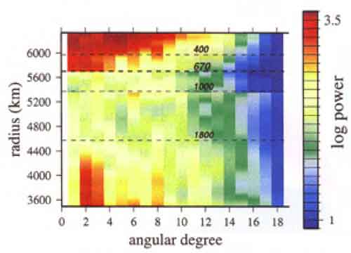 Spherical harmonic power spectrum of velocity throughout the mantle (from Gu et al., 2001). The Earth is clearly characterised by strong heterogeneity in the longer-wavelength components in the lithosphere and upper mantle and the lowermost mantle, with little heterogeneity in between. The three major regions of the mantle are evident. There may also be chemically distinct layers at the very base of the mantle (D") and a buoyant, refractory layer at the top of the mantle (the perisphere).
 |
The forces on plates
The creation of new plates at ridges, the subsequent cooling of these plates, and their ultimate subduction at trenches introduce forces which drive and break up the plates. They also introduce chemical and thermal inhomogeneities into the mantle. Plate forces such as ridge push, slab pull, and trench suction are basically gravitational forces generated by cooling plates. They are resisted by transform fault, bending and tearing resistance, mantle viscosity and bottom drag. If convection currents dragged plates around, the bottom drag force would be the most important. However, there is no evidence that this is a strong force, and even its sign is unknown (driving or resisting drag). The thermal and density variations introduced into the mantle by subduction also generate forces on the plates. The deep mantle, even if convectively isolated from the upper mantle, affects the elevation and stress state of the lithosphere. Density variations in the mantle also cause variations in elevation and stress in the plate, which are added to the plate forces. Hot regions of the lower mantle will heat the upper mantle and may control, to some extent, the locations of supercontinents and long-lived subduction zones. Even if the mantle is irreversibly chemically stratified into two or more layers, the deep layers will have an effect on geophysical observables. Regions of high elevation, tensile stress and volcanism will tend to be above low-density regions of the deep mantle unless counteracted by gravitational forces in the plates themselves and at plate boundaries. Because of the high viscosity of the deep mantle the warm regions are semi-permanent compared to features in the upper mantle. The large viscosity contrast means that the various layers are more likely, on average, to be thermally coupled than shear coupled. From a tomographic point of view, this means that some mantle structures may appear to be continuous even if the mantle is stratified (see (11) and http://karel.troja.mff.cuni.cz/staff/HANKA_CIZKOVA/Anim/animace.htm). |
The core-mantle boundary region
The TBL at the base of the mantle generates a potentially unstable situation. The effects of pressure increase the thermal conductivity, decrease the thermal expansion and increase the viscosity. This means that conductive heat transfer from below is more efficient than at the surface, that temperature increases have little effect on density and that any convection will be sluggish. Although the amount of heat coming out of the core may be appreciable, it is certainly less (~10%) than that flowing through the surface. The net result is that lower-mantle upwellings take a long time to develop and they must be very large in order to accumulate enough buoyancy to overcome viscous resistance. The spatial and temporal scale of core-mantle-boundary instabilities are orders of magnitude larger than those at the surface. This physics is not captured in laboratory simulations or calculations that adopt the popular Boussinesq approximation. Pressure also makes it easier to irreversibly chemically stratify the mantle. A small intrinsic density difference due to subtle changes in chemistry can keep a deep layer trapped since it requires such large temperature increases to make it buoyant. Layered mantle convection is the likely outcome. |
A Primer on Convection A system cooled from above or heated from within will develop an upper thermal boundary layer which drives the system. The thermal boundary layer (plate, slab) is the only active element. All upwellings are passive, and diffuse. For large Prandtl number (the mantle) the mechanical boundary layers are the size of the mantle. The scale of thermal boundary layers (plate thickness) is controlled by the Rayleigh number (Ra), which for the top is of the order of hundreds of km. Ra is controlled both by physical properties (conductivity, expansivity etc.) and environment (heat flow, temperature gradients etc.). Both these factors cause Ra to be orders of magnitude lower at the base of mantle than at top. Therefore convective vigor is orders of magnitude less at the base of mantle. The mechanical and thermal boundary layers at the base of mantle are therefore of the order of thousands of kilometers in lateral dimensions. Radioactivity does not contribute to unstable superadiabatic gradients because the time constants are much greater than convective time constants. |
|
|
Notes
In the Morgan plume theory, upwellings are the active narrow elements and downwellings are passive and diffuse. This is the exact opposite of cooled-from-above-systems and what the geophysical data tell us. Morgan plume theory holds for systems heated from below and not cooled from above.
If there are no pressure effects and if all the heat enters from below and leaves from the top then there is symmetry and both upper and lower TBL are active.
Sphericity, pressure, continents and distribution of radioactivity break symmetry and mean that lower TBL instabilities are sluggish and gigantic compared with upper TBL instabilities (slabs).
Continents/cratons also contribute to the lateral thermal gradients that drive convection from the top.
It is lateral thermal gradients, not vertical ones, that drive convection.
The lithosphere, instead of the mantle, controls cooling of mantle. |
References - M. Gurnis, Nature, 332, 695 (1988).
- M. Gurnis, S. Zhong, Geophys. Res. Lett., 18, 581 (1991).
- M. Gurnis, S. Zhong, J. Toth, The history and dynamics of global plate motions, AGU, Geophysical Monograph 121, pp. 73, (2000)
- J. P. Lowman, G. T. Jarvis, Geophys. Res. Lett., 20, 2087 (1993).
- J. P. Lowman, G. T. Jarvis, J. Geophys. Res., 104, 12,733 (1999).
- S. Zhong, M. Gurnis, Geophys. Res. Lett., 22, 981 (1995)
- Anderson, D. L., Top-down tectonics, Science, 293, 2016 (2001).
- Anderson, D. L., A statistical test of the two reservoir model for helium, Earth Planet. Sci. Lett., 193, 77 (2001).
- Anderson, D. L., 2001, How many Plates?, Geology, 30, 411 (2002).
- Anderson, D. L. Plate Tectonics as a Far- From- Equilibrium Self-Organized System, in Plate Boundary Zones, ed. S. Stein, AGU Monograph, (2002).
- Cizkova, H., Cadek, O., van den Berg, A.P. and N.J. Vlaar, Can lower mantle slab-like seismic anomalies be explained by thermal coupling between the upper and lower mantles? Geophys. Res. Lett., 26, 1501-1504, 1999.
General References
- Agee, C. B. and Walker, D., Mass balance and phase density constraints on early differentiation of chondritic mantle, Earth Planet. Sci. Lett., 90, 144 (1988).
- Anderson, D. L., Theory of the Earth, Blackwell Scientific Publications, Boston, pp. 366 (1989). [Chapter 8 is relevant to irreversible stratification of mantle and low U in the lower mantle.]
- Anderson, D. L., Where on Earth is the Crust?, Physics Today, March 1989, 38-46. (1989).
- Clark, S. P., and Turekian, K. K., Thermal constraints on the distribution of long-lived radioactive elements in the Earth: Phil. Trans. R. Soc. Lond., 291, 269-275 (1979).
- Coltice, N., and Ricard, Y., Geochemical observations and one layer mantle convection: Earth Planet. Sci. Lett., 174, 125-137 (1999).
- Conrad, C. P., and Hager, B. H., Mantle convection with strong subduction zones: Geophys. J. Int., 144, 271-288 (2001).
- Cordery, M. J., Davies, G. F., and Campbell, I. H., Genesis of flood basalts from eclogite-bearing mantle plumes: J. Geophys. Res., 102, 20,179-20,197 (1997).
- Cserepes, L., Yuen, D. A., and Schroeder, B. A., Effect of the mid-mantle viscosity and phase-transition structure of 3D mantle convection: Phys. Earth. Planet. Int., 118, 135-148 (2000)
- Davaille A., Simultaneous generation of hotspots and superswells by convection in a heterogeneous planetary mantle: Nature, 402, 756-760 (1999).
- Davies, G. F., Dynamic Earth: Plates, Plumes and Mantle Convection: Cambridge University Press, Cambridge, 458 pp. (2000).
- Gu, Y., A.M. Dziewonski, S. Weijia, and G. Ekstrom, Models of the mantle shear velocity and discontinuities in the pattern of lateral heterogeneities, J. geophys. Res., 106, 11,169-11,199 (2001).
- King, S. D., and Anderson, D. L., An alternative mechanism of flood basalt formation: Earth Planet. Sci. Lett., 136, 269-279 (1995).
- Ritsema, J., H.J. van Heijst, and J.H. Woodhouse, Complex shear wave velocity structure imaged beneath Africa and Iceland, Science, 286, 1925-1928 (1999).
- Schubert, G., Turcotte, D., Olson, P., Mantle convection in the Earth and planets: C. U. Press, 956 pp. (2001).
- Scrivner, C. and Anderson, D. L., The effect of post Pangea subduction on global mantle tomography and convection: Geophys. Res. Lett., 19, 1053-1056 (1992).
- Tackley, P. J., Mantle convection and plate tectonics: Toward an integrated physical and chemical theory: Science, 288, 2002-2007 (2000).
- Tackley, P., Three dimensional simulations of mantle convection with a thermo-chemical basal boundary layer: in: M. Gurnis, M. et al., eds., The Core-Mantle Boundary Region, Washington, AGU, 334 pp. (1998).
- Turcotte, D.L. and G. Schubert, in Geodynamics, John Wiley & Sons, New York, 450 pp. (1982).
- Wen, L. and Anderson, D. L., Layered mantle convection: A model for geoid and topography: Earth Planet. Sci. Lett., 146, 367-377 (1997).
- Wen, L. and Anderson, D. L., Slabs, hotspots, cratons and mantle convection revealed from residual seismic tomography in the upper mantle: Phys. Earth Planet. Int., 99, 131-143 (1997).
- http://jspc-www.colorado.edu/~szhong/mantle.html
|

 ,
,  , and
, and  respectively. The Fourier transform has the following basic properties (Pinsky 2002).
 .
. . The case a = −1 leads to the time-reversal property, which states: if h(x) = ƒ(−x), then
  .
. , then


 , then

 per q = 0, 1, ..., N-1